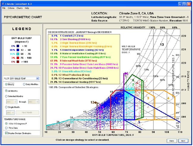
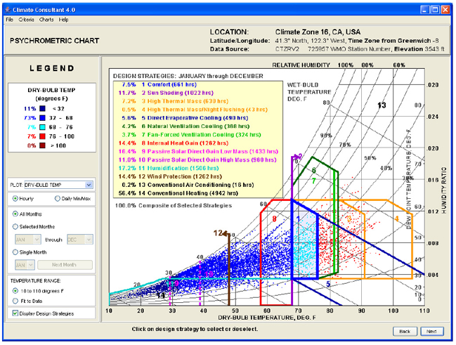
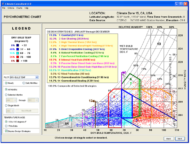
To further compare results with these tools a single family dwelling was analyzed in four climates. This dwelling was two stories high and 48 by 24 ft, with 2300 sq ft gross building floor area, which is close to the 2005 US average. The four climates regions were: a) HOT AND DRY: California climate zone 15 (El Centro); COLD: California climate zone 16; TEMPERATE: California climate zone 6 (Los Angeles); and HOT AND HUMID: Miami, Florida. The psychrometric charts in figures 3,4,5 and 6 illustrate the conditions in these climates. Much more extreme climates (warmer in the hot climates or colder in the cold climates) for each of these could have been selected but these were deemed as representative without being too extreme.
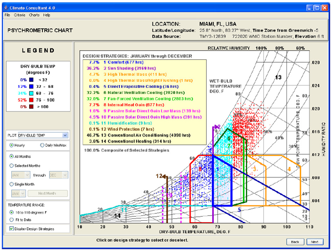
Figure 6: Psychrometric chart for the Hot Humid Climate (Miami)
Several assumptions were made for each of the areas in which buildings emit carbon (operational energy, construction, waste, water and transportation) and are explained in the following sections.
4.1 Operational Energy
Title 24 was used to define the building envelope for all climate zones. Package D for homes with natural gas was used. The same envelope requirements were used for hot and humid and hot and dry climates (Table 4).
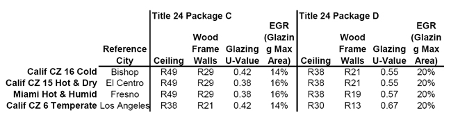
TABLE 4: ENVELOPE CHARACTERISTICS
Operational energy includes all the energy to keep the buildings and everything inside it running. According to Bordass (5) the process to estimate CO2 emissions from operational energy use in buildings involves five steps:
1. Define the boundary of the premises. Boundaries should be where they make practical sense in terms of where the energy can be counted (e.g. the area fed by the meters) and how the area is run (a tenancy, a building, a site; or even a district or a city). One may look at more than one boundary, e.g. for a university the campus, specific buildings, and individual departments; and for a rented building the whole building, and each tenancy.
2. Measure the flows of each energy supply across the defined boundary. Normally this will be annual totals by fuel, though details of load profiles could sometimes be included.
3. Define carbon dioxide factors for each energy supply.
4. Multiply each energy flow by the appropriate carbon dioxide facto to get the emissions associated with each fuel.
5. Add them up. to get the annual total of CO2 emissions.
To calculate the CO2 factors for each energy supply we must determine the emission factors for each one. There are several methods to determine these factors (6):
- The EPA Power Profiler – calculates CO2 emission factors for historical yearly average emissions for every U.S. zip code.
- The EPA eGRID – a database that has hourly CO2 emissions for every U.S. power plant. However, this data is also historical and it is a non-trivial task to estimate marginal generation from this database.
- The NREL Model – they developed direct and indirect impacts for typical building fuels and used CO2 e (equivalent) which includes other important GHG besides CO2 , like methane (CH4 ) and nitrous oxide (N2 O). This model generated emission factors for all U.S. regions as well as the nation.
- The CEC/E3 Model – used the output of a production simulation dispatch model to forecast average and marginal CO2 emission factors for California.
Because different locations would use different electrical and gas utilities which would further muddle the numbers, the same values were used for electricity and gas in all the projects: 1.363 lbs of CO2 per kWh for electricity, which is the average value for the United States and 11.924 lbs of CO2 per therm for gas.
4.2 Construction
Carbon emissions from construction processes are usually generated a) during the fabrication of the materials used in the building, b) during transportation of materials to the building and c) during construction of the building. Construction related emissions are usually more difficult to calculate because it is not easy to determine with precision the manufacturing process, origin, and transportation modes of the materials from its place of origin to the site. It is also difficult to determine the amount of each material in the building.
Emissions for construction were calculated using buildcarbonneutral, (7) a very simple calculator that provides rough results. More precise data can be generated using Athena Ecocalculator for assemblies. However this is not available for all regions.
The following input was provided to the calculator to determine emissions due to construction materials: floor area of 2300 sq ft, two stories high, structural wood system, Mediterranean California ecoregion, previously developed existing vegetation, short grass installed, disturbed landscape of 6500 sq ft and 1500 sq ft installed. The total emissions from construction were 53 metric tons or 116,812 lbs. of C02 / year. We estimated a building lifespan of 50 years, which is equivalent to 2336.2 lbs/year over the life of the building. If construction components could be recycled or the life of the building could be extended then the impact would be lower. If the building required major renovations then construction related CO2 emissions would be higher. The same number was used in the building in all sites.
4.3 Waste
Waste generated from the building must also be treated. More waste requires more treatment and sometimes generates methane, which is a potent greenhouse gas produced in landfills.
To determine emissions due to waste, we used the waste portion of the carbon emissions calculator developed by the EPA (8). We assumed that the home recycled 50% of its waste (plastic, aluminum, newspapers, glass, magazines, etc.) This reduced the emissions from 1,021 lbs of CO2 per year / per person to 574 lbs of CO2 per year / person. Since we assumed a household of four we assumed this generated 2,296 lbs of CO2 / dwelling / year from waste . This value was also assumed equal in all locations.
4.4 Water
Water provided to the building and coming from the building must also be treated in a process which usually is also responsible for the generation of CO2 emissions. The water that is used in the building must be pumped from the source, then treated to be made potable, and then pumped to the building for consumption. The waste water from the building must also be treated, which also generates carbon emissions by using energy for these processes.
A study on Water-Related Energy Use in California by the Assembly Committee on Water, Parks and Wildlife (9) calculated the water embedded energy for southern and northern California. They estimated the amount of energy needed for each sector of the water-use cycle in terms of the number of kilowatt-hours (kWh) needed to collect, extract, convey, treat, and distribute one million gallons (MG) of water, and the number of kWh needed to treat and dispose of the same quantity of wastewater. For Southern California the embedded energy per MG is 13,021 kWh. We used these numbers to estimate the energy embedded in the water for a family of four that would use 400 gallons of water per day. This means that to provide 146,000 gallons a year to a family of four in southern California would require 1901 kWh. If every kWh of electricity in California generates about 0.7 lbs of CO2 (4) then the average water use for a family of four generates about 1,331 lbs of C02 / year. This number was used for all sites even though the number for southern California is higher than the number for Northern California and probably higher than for the rest of the United States.
4.5 Transportation
A building is also indirectly responsible for CO2 emissions from transportation. By its location it affects how the building users move to and from the building. A location close to public transit lines or in urban areas with higher density and walkable neighborhhoods usually reduces transportation related carbon emissions.
We assumed that each household drove a total of 15,000 miles per year in cars with 22 MPG efficiency. A factor of 19.5 lbs of CO2/Gal (10) was used. A total yearly value of 13,295 lbs of CO2 per year for transportation from the home was determined. This value could be assigned to the home, work or divided between both. We assigned this value to the home.
We did not include carbon emissions for air travel because these are not affected by the location of the residence.